
uv, part 4: uv with Jupyter
Using uv with Jupyter: demo using polars and seaborn for analysis and visualization.
This is part 4 of a series on uv. Other posts in this series:
I’ve never been a big fan of notebooks, and I’m not the only one. Out of order code execution, hidden state, difficulty diffing in version control, output bloat, etc. are all factors that make me prefer Quarto instead of notebooks.
However, notebooks are still useful for interactive exploration and data analysis. And you’ll inevitably encounter notebooks in computational biology. Many of the GitHub repos in the papers I summarize each week are notebooks demonstrating a certain analysis, training a particular model, etc.
Here I’ll show you how to use uv with Jupyter, demonstrating how to do some dplyr and ggplot2-like summary analysis and visualization inside a Jupyter notebook using polars and seaborn.
Demo
You can see the full rendered notebook for this demo here on GitHub.
Start Jupyter Lab with uv
uv makes it easy to set up Jupyter notebooks, either to interact with a project or to use as a standalone tool. The docs on using uv with Jupyter are helpful in understanding that distinction and how the kernel and dependencies either hook into the project’s virtual environment or the project dependencies. Here I’m going to install packages into the notebook environment without creating a kernel, so that installed packages run in an isolated environment within the notebook itself.
To start a Jupyter Lab session with uv, this is all you need. This will set up an isolated environment with jupyter installed, and will run jupyter lab.
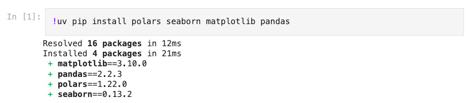
uv run --with jupyter jupyter labI’m going to be using polars, seaborn, matplotlib, and pandas in this demo. So the first thing I’ll do in my notebook is run a shell command to install some of those dependencies inside the notebook environment with uv.1 Notice that this takes only a few milliseconds.
Data analysis with polars
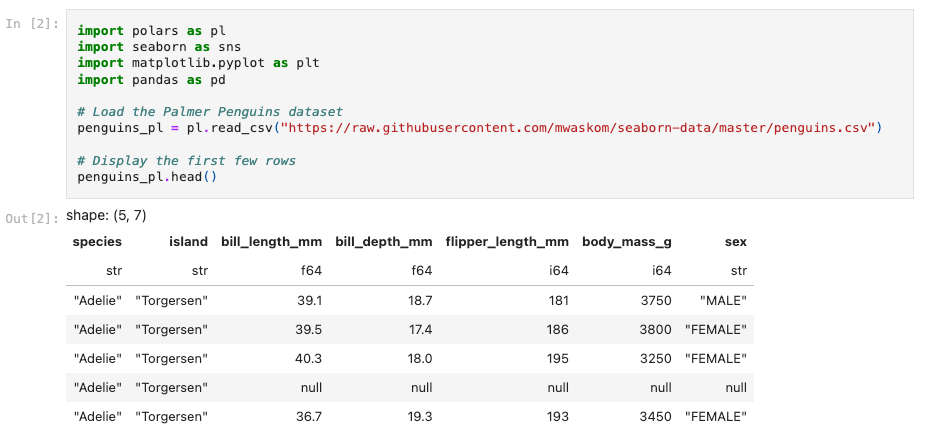
Next I’m going to import those packages, read in the Palmer penguins data from the seaborn examples repo, and show a few rows.
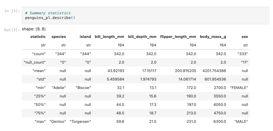
I can also get some summary information about each column.
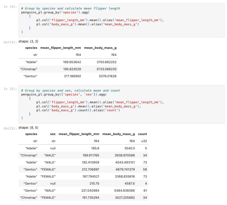
I can do dplyr-like operations. Here I’m grouping by species and calculating mean flipper length and body mass, then grouping by species and sex and calculating the mean flipper length and body mass and counts for each group.
Visualization using seaborn
In the last chunk I’m converting the polars data frame back to a pandas data frame so I can use seaborn for plotting. I’ll then make a scatterplot colored by species, with the sex mapped onto the point shape, similar to aes(color=species, shape=sex) if you were using ggplot2.

Here’s the resulting plot:

You can see the full rendered notebook for this demo here on GitHub.
Resources
Last year I wrote a post with resources for learning Python as an R user:

In that post I recommended several of Emily Riederer’s posts on Python Rgnomics — tools, packages, infrastructure, etc. for coming to Python from the R world. Since I wrote that post, Emily updated this with her Python Rgonomics - 2025 Update post, which I strongly recommend reading (where she recommends uv, polars, seaborn, etc.).
See also the previous posts in this series. Using scripts and tools:

Building and publishing packages:

Python in R with reticulate:

Finally, don’t skip over the official docs on using uv with Jupyter.
Yes, I could have avoided the need to install additional dependencies in my notebook with: uv run --with jupyter,polars,seaborn,matplotlib,pandas jupyter lab. This would have started the uv environment with all the dependencies my notebook needed, not just jupyter.